Continuous Futures Historical Data for Eurodollar Adjustment Method
Welcome! If you enjoy these posts, please follow this blog via email and check out my Twitter feed located on the sidebar.
All of my previous analysis has focused on US equities, but today we begin the journey into another asset class, futures. Futures are traded via contracts where two parties agree to exchange a quantity of an asset for a price decided today and delivered at a specified date in the future. The expiration dates of the contracts vary based on the underlying asset and range from monthly to quarterly. To properly evaluate the profitability of trading strategies with historical futures contract data, it is necessary to combine these contracts into a continuous price series. This isn't entirely straightforward because contango and backwardation factors cause contracts of the same underlying asset with different expiration dates to be priced differently. It is initially unclear how to best concatenate these price series, so I want to explore a few of the basic methods and their advantages. I'm interested in exploring futures strategies, so this was a necessary first step since Quandl's free continuous futures data is of insufficient quality, but they provide high quality individual contract data. Becoming comfortable with the contract data while creating flexible, testable continuous price series is a valuable exercise. Additionally, I decided to use Python because I have not done a project with it and this is a useful applied problem to build some Python skills.
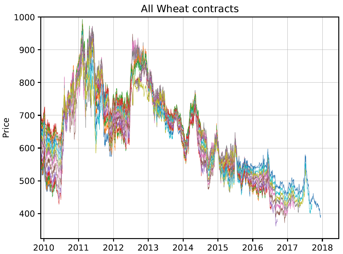
For this example, we will construct a variety of continuous price series for the commodity wheat. The first step is to pull the contract data from the Quandl API and store it appropriately (see the included code). To begin, let's plot all the contracts' prices to observe the behavior of the price data. As seen in Figure 1 below, although there is some consistency between the contracts, there is a significant amount of variance.
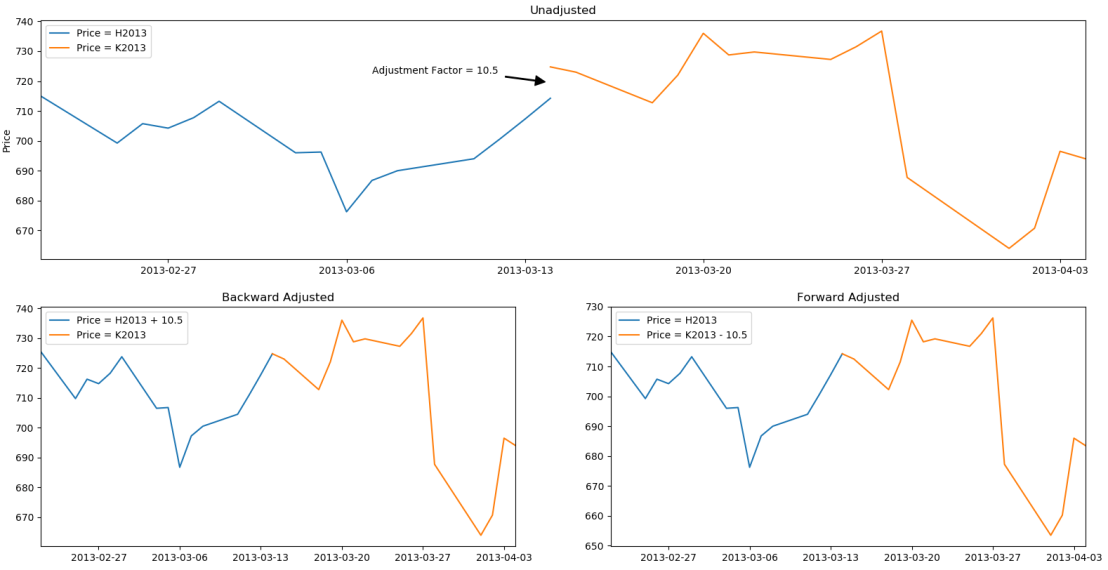
Ideally, to make this a backtest-ready series, we need to be trading a single contract at each point in time (or possibly a combination of contracts). The further we are from a contract's expiration; the more price speculation is embedded into the price. The front or nearest month contract refers to the contract which has the soonest expiration date and thus has the least amount of speculation. Generally, front month contracts have the most trading activity, as measured by open interest. When expiration approaches, traders will roll their positions over to the next contract or let them expire. A basic approach to construct a continuous series would be to always use the front month contract's price and when the current front month contract expires, switch to the new front month contract. There is one caveat, the price of the contracts when you rollover may not be the same, and in general, won't be the same. These gaps will create artificial, untradeable price movements in the continuous series. To create a smooth transition between contracts, we can adjust them in such a way so that there won't be a gap. We'll refer to the size of this gap as the adjustment factor. Forward adjusting would shift the next contract to eliminate the gap by subtracting the adjustment factor from the next contract's price series. Backward adjusting would shift the previous contract to eliminate the gap by adding the adjustment factor to the previous contract's price series. Figure 2 below shows an example of these adjustments for an actual rollover.
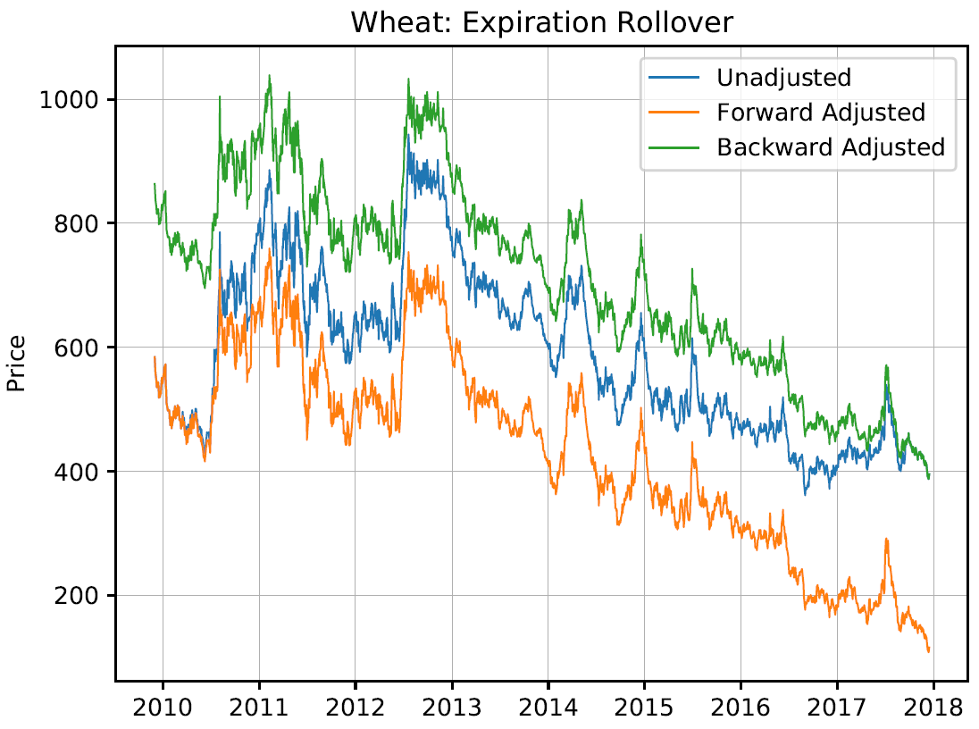
Now, when this approach is extended over multiple contracts the adjustment factors will simply cumulate so that prices for every contract are appropriately adjusted. The quality of the data is the same whether you backward or forward adjust. The difference is what needs to be recalculated with each new contract and what the values represent. The backward adjusted series' current values represent the actual market values thus the historical data needs to be recalculated when a new contract is added to the series. The forward adjusted series does not require recalculating historical data but since each new contract that is added to the series needs to be adjusted, the new prices will not represent the actual market values. Figure 3 below shows the fully adjusted wheat series. Notice that the difference between the forward and backward adjusted series remains constant. This difference is the total adjustment factor.
A point that becomes apparent, here, is that we are adjusting the price series, not the returns. The daily returns of the forward and backward adjusted series differ. When creating continuous prices, you are forced to choose between either correct P&L or correct returns. To adjust for correct returns, one would need to work with the daily log returns series of the contracts and then construct a usable price series from those. Dr. Ernest Chan's second book covers this concept thoroughly on pg. 12-16.
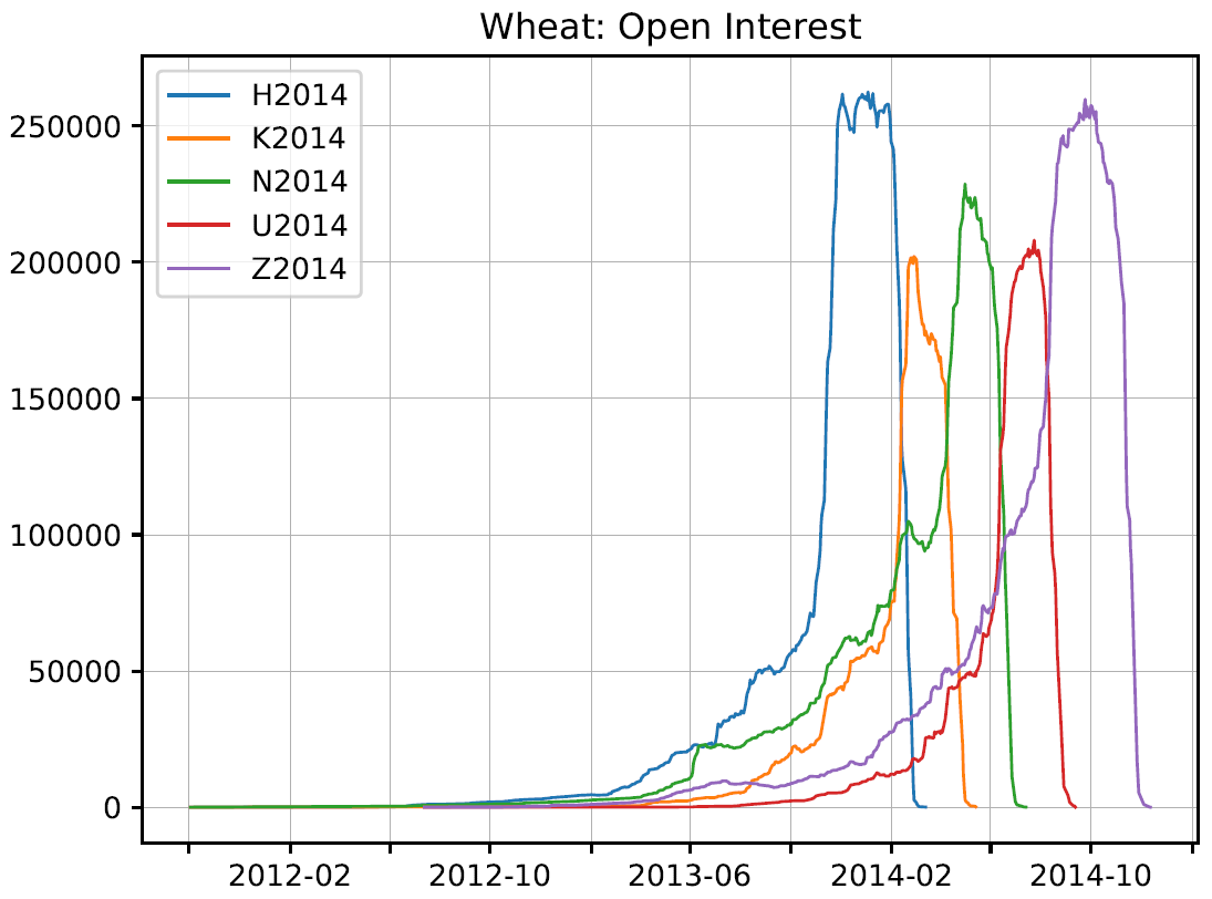
Another approach to construct a continuous series is the perpetual method, which smooths the transitions between contracts by taking a weighted average of the contracts' prices during the transition period. This can be weighted on time left to expiration, open interest, or other properties of the contracts. For this example, we will begin the transition to the next contract once its open interest becomes greater than the current contract and weight the prices during the transition based on open interest. As seen in Figure 4 below, this happens prior to the expiration of the contracts.
Like the previous example, one could also forward/backward adjust using the open interest crossover date which is more realistic because of better liquidity. This option is available in the attached code. In our case, after this crossover date, we transition to the next contract over the next 5 days (the number of days is adjustable) based on open interest. Figure 5 below shows the slightly smoother perpetual adjusted series.
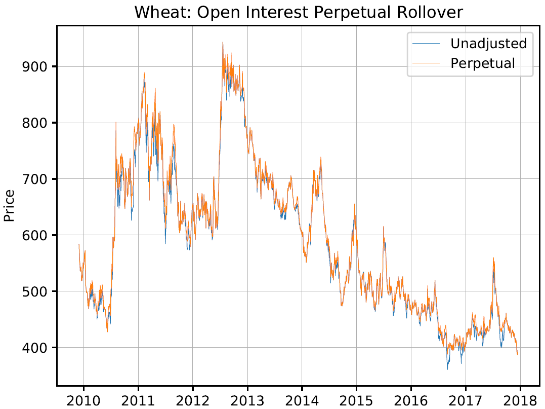
This smoothed price series may be advantageous for statistical research since it reduces noise in longer term signals but it contains prices that are not directly tradable. To trade the price during the transition period, one would have to rebalance their percentage of the current and next contract each day, which would incur transaction costs.
There are a variety of other adjustment methods, but the examples shown here provide a strong and sufficient foundation. A paper that I found very helpful and one that covers additional methods is available here. The Python code accompanying this post can be found here. I hope you found these examples helpful. In my next post, I am going to use these continuous series as I analyze futures trading strategies. Thanks for reading!
Source: https://quantoisseur.com/2018/02/05/constructing-continuous-futures-price-series/
0 Response to "Continuous Futures Historical Data for Eurodollar Adjustment Method"
Enviar um comentário